Original content by the OOTEE Optics editorial team, drawn from first-hand production line and inspection data. Please credit the source when republishing.
Given limits in expertise and test conditions, the theories, parameters and conclusions here carry no guarantee of absolute accuracy. For technical learning and exchange only - never the sole basis for design, acceptance or selection. Corrections welcome.

A filter’s diameter or rectangular outline sets a mechanical boundary. Together with thickness and clear aperture, it determines whether the beam passes without clipping, how the optic behaves in its mount, and which parts of a test report describe actual operation.
An ideal, spatially uniform coating does not acquire a different center wavelength (CWL) or full width at half maximum (FWHM) simply because its substrate is wider. Practical size effects arise when the illuminated region expands, samples more coating variation, or becomes more sensitive to support conditions, so a large part rarely measures exactly like a small coupon cut from the same run.
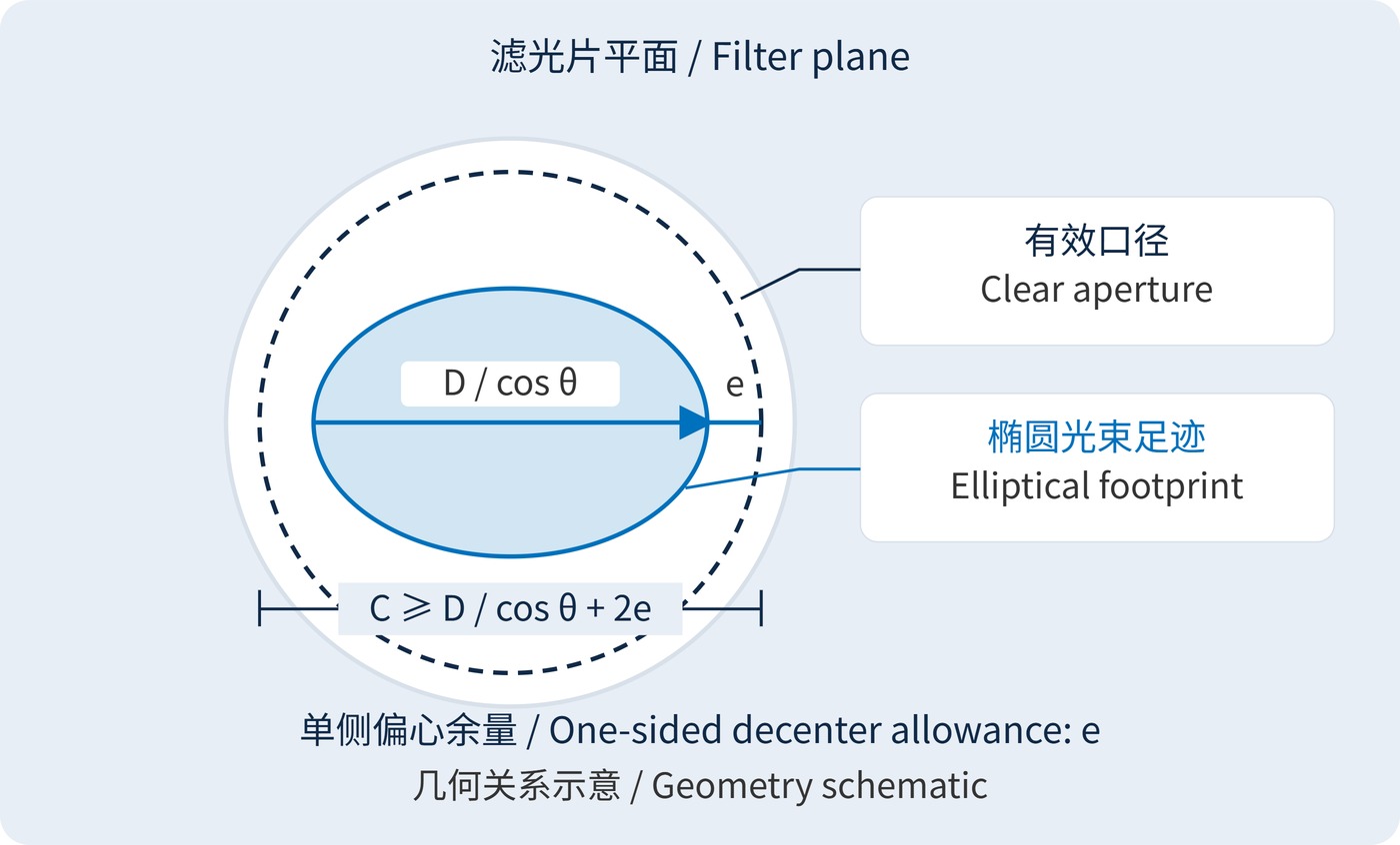
Start with the projected footprint. As Fig. 1 shows, a circular collimated beam produces an ellipse on a tilted filter. For beam diameter $D$ measured perpendicular to propagation, angle of incidence (AOI) $\theta$, and a one-sided lateral allowance $e$, the required clear aperture along the ellipse’s major axis is:
$$C_{\mathrm{req}} \geq \frac{D}{\cos\theta}+2e$$
This is a projection model for a collimated beam on a plane. Converging cones, field-dependent movement and barrel restrictions require separate ray tracing. The allowance is measured in the filter plane and covers decenter and position drift. For a Gaussian beam, define an acceptable enclosed-power boundary first: its $1/e^2$ diameter is not a hard edge.
Next consider spatial averaging. When local spectra differ across a coating, a detector collecting the transmitted beam measures an irradiance-weighted response. At a fixed AOI, with incoherent power addition and full collection of transmitted power:
$$T_{\mathrm{eff}}(\lambda)=\frac{\int_A I(x,y,\lambda)T(x,y,\lambda)\,\mathrm{d}A}{\int_A I(x,y,\lambda)\,\mathrm{d}A}$$
Here $A$ is the illuminated region accepted by the system. Offset local passbands can broaden the combined response or reduce its peak. Edge variation contributes little if only the center is illuminated. Account for clipping separately; normalizing a spectrum to the surviving beam can conceal lost throughput.
Optical density (OD) follows $\mathrm{OD}=-\log_{10}T$, with $T$ expressed as a power fraction. Do not average local OD values: average transmission with the appropriate weights, then convert. A wide, thin substrate may also be more sensitive to coating stress and clamping. Mounted transmitted-wavefront measurements establish whether this matters for imaging.
Consider a 12 mm collimated beam at 30° AOI with a 1 mm allowance on each side. The required clear aperture is approximately 15.9 mm. If only 85% of the outer diameter is guaranteed clear, the preliminary diameter limit is about 18.7 mm. Retainer openings, bevels and negative dimensional tolerances still need checking.
For a narrow bandpass filter targeting CWL 780 nm, FWHM 20 nm and OD6 blocking, specify the blocking wavelength interval, AOI, cone angle and guaranteed aperture together. These are example requirements, not a claim of available stock performance. A diameter and a passing center scan leave too much undefined.
| Acceptance item | Conditions to specify |
|---|---|
| Throughput and fit | Minimum clear aperture, retainer opening, decenter and full-field beam envelope |
| Spatial spectra | Center and edge-zone coordinates, spot size, local CWL and FWHM limits |
| Blocking | Minimum OD over a stated interval, instrument dynamic range and stray-light control |
| Mechanics and imaging | Thickness, supports, clamping conditions and mounted transmitted wavefront |
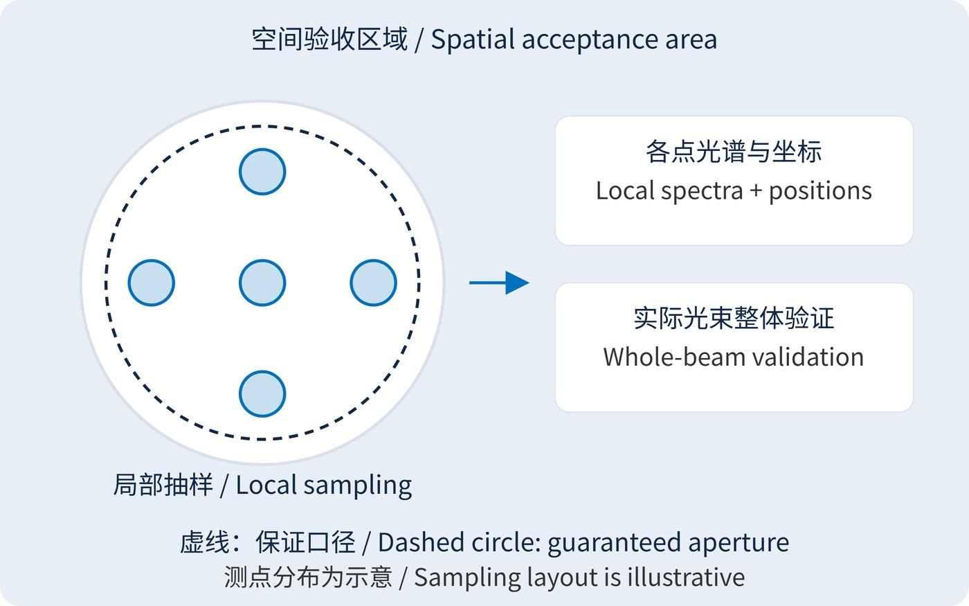
Fig. 2 shows a useful starting pattern: one center position and four edge-zone positions. Five samples cannot certify every location. Keep each test spot fully within the guaranteed area, increase sampling density to resolve spatial changes, and add a full-aperture test using the intended beam for demanding narrowband or large-area illumination.
A filter ahead of a machine-vision lens can experience footprint movement across the field. Insufficient aperture creates vignetting; spatial spectral variation may produce brightness or color differences. Evaluate machine vision filters at the widest required field and operating aperture, including the corners of the image.
In fluorescence collection and laser receivers, a larger opening can accept more light only if the remaining stops and detector support it. Increasing the accepted angular range introduces another variable. Separate spatial variation from AOI effects before attributing a spectral change to diameter.
Close the specification loop by deriving aperture from the beam envelope, defining acceptance over that aperture, and verifying the response under the intended illumination and support conditions.
 365nm Narrow Bandpass Filter | Ø50mm | T>90%
OT-HBP3659050
365nm Narrow Bandpass Filter; FWHM 10nm; transmission >90%; blocking OD5; size Ø50mm; AOI 0°.
 450nm Narrow Bandpass Filter | Ø50mm
OT-HBP4509050
450nm Narrow Bandpass Filter; FWHM 10nm; transmission >90%; blocking OD5; size Ø50mm; AOI 0°.
 525nm Narrow Bandpass Filter | Ø50mm
OT-HBP5259050
525nm Narrow Bandpass Filter; FWHM 10nm; transmission >90%; blocking OD5; size Ø50mm; AOI 0°.
Send us your drawing and spectral targets — an engineer replies with a feasibility check and quotation within one business day.