Original content by the OOTEE Optics editorial team, drawn from first-hand production line and inspection data. Please credit the source when republishing.
Given limits in expertise and test conditions, the theories, parameters and conclusions here carry no guarantee of absolute accuracy. For technical learning and exchange only - never the sole basis for design, acceptance or selection. Corrections welcome.
A transmission plot and a blocking plot may describe exactly the same filter data. The distinction often lies in the vertical axis: percentage transmission emphasizes useful light, while optical density (OD) makes small leakage visible. Reading them together is a coordinate-reading exercise before it becomes a filter-selection exercise.
Start with the wavelength axis, normally in nm, and check whether the vertical scale shows %, fractional transmission, or OD. High transmission and high OD mean opposite things. Also, blocking does not identify where the rejected energy goes: a transmission plot alone cannot separate reflection from absorption.
Transmission is the ratio of transmitted to incident optical power at a given wavelength. Use a fraction between 0 and 1 when calculating OD:
$$\mathrm{OD}(\lambda)=-\log_{10}T(\lambda),\qquad T(\lambda)=\frac{P_{\mathrm{out}}(\lambda)}{P_{\mathrm{in}}(\lambda)}$$
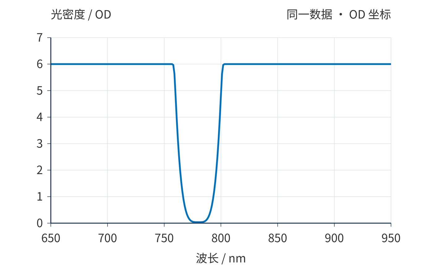
Thus 1% is OD2, 0.01% is OD4, and 0.0001% is OD6. On a 0–100% plot, the last two values are practically indistinguishable from the baseline. Fig. 1 is useful for examining the passband shape, but its apparent zero cannot establish deep blocking.
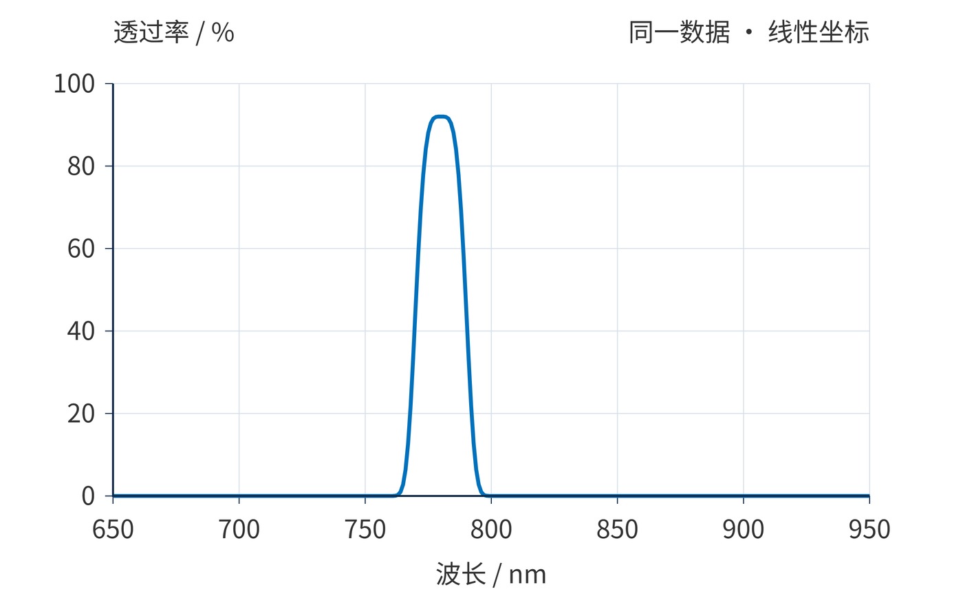
The example has a center wavelength (CWL) of 780 nm and a full width at half maximum (FWHM) of approximately 20 nm. With a 92% peak, half maximum is 46%, rather than an absolute transmission of 50%. For this symmetric single peak, the midpoint of the half-height crossings also locates the center. An asymmetric or multiple-peak spectrum needs an explicit CWL definition.
$$T(\lambda_1)=T(\lambda_2)=\frac{T_{\mathrm{peak}}}{2},\qquad \mathrm{FWHM}=\lambda_2-\lambda_1$$
Both figures are calculated from the following illustrative function, with wavelength expressed in nm. This is a reproducible reading example, rather than a thin-film simulation or a product specification:
$$T(\lambda)=10^{-6}+(0.92-10^{-6})\exp\left[-\ln 2\left(\frac{\lambda-780\,\mathrm{nm}}{10\,\mathrm{nm}}\right)^4\right]$$
In Fig. 2, the transmission peak becomes an OD minimum. At 780 nm, OD is about 0.036; at 770 and 790 nm it is about 0.337. Farther from the passband, the curve approaches OD6. The reversed appearance comes entirely from the logarithmic conversion.
Locate the wanted signal and unwanted light on the wavelength axis first. Then read transmission within the signal window and OD within each specified blocking window. A transition region should not be treated as representative of the entire stopband. The following requirements are a reading exercise, with no associated product model.
| Region | Example requirement | What to inspect |
|---|---|---|
| Signal window | 775–785 nm; transmission ≥85% | Lowest transmission across the window |
| Band location | CWL 780 nm; FWHM 20 nm | Crossings at half the actual peak |
| Blocking windows | 650–750 nm and 810–950 nm; OD ≥6 | Lowest OD across both windows |
The ideal curve meets the illustrative passband requirement. Its blocking approaches OD6, however, so it cannot establish that a physical filter meets OD ≥6. Check angle of incidence (AOI), polarization, temperature, and beam geometry as well. A spectrum measured at AOI 0° does not establish acceptance at 15°. Measurement uncertainty also needs margin against the limit.
When reviewing a purchasing attachment, keep both views together and compare identical wavelength spans. A magnified peak and a separate remote blocking plot can leave the transition unreported. Request the missing interval rather than mentally connecting the traces. Preserve unsmoothed data when smoothing is used: a narrow leakage feature can disappear in presentation processing. The width of a plotted line is not a performance tolerance.
For near-infrared imaging, use the linear plot to check illumination near 780 nm, then inspect blocking wherever the detector remains sensitive. If detector response extends beyond 1000 nm but the plot ends at 950 nm, the missing region remains unknown. Extending the final plotted value would create unsupported data.
In weak fluorescence measurements, inspect the excitation wavelength separately from the emission window. A small transmitted fraction of a strong excitation source can still dominate a weak signal. Broadband background requires consideration of source spectrum and detector response; OD at one wavelength does not describe integrated leakage.
Stray light and measurement error depend on instrument calibration, spectral bandwidth and sample condition. A defensible interpretation aligns the axis, wavelength coverage, measurement conditions, and acceptance limits.
 365nm Narrow Bandpass Filter | Ø50mm | T>90%
OT-HBP3659050
365nm Narrow Bandpass Filter; FWHM 10nm; transmission >90%; blocking OD5; size Ø50mm; AOI 0°.
 450nm Narrow Bandpass Filter | Ø50mm
OT-HBP4509050
450nm Narrow Bandpass Filter; FWHM 10nm; transmission >90%; blocking OD5; size Ø50mm; AOI 0°.
 525nm Narrow Bandpass Filter | Ø50mm
OT-HBP5259050
525nm Narrow Bandpass Filter; FWHM 10nm; transmission >90%; blocking OD5; size Ø50mm; AOI 0°.
Send us your drawing and spectral targets — an engineer replies with a feasibility check and quotation within one business day.